 Login/Register


Curve Fitting for Immunoassays: ELISA and Multiplex Bead Based Assays (LEGENDplex™)
| Our LEGENDplex™ flow cytometry-based multiplex immunoassays quantify multiple soluble analytes simultaneously in several biological samples. Using the same basic principles of sandwich immunoassays. LEGENDplex™ uses common lab flow cytometers for data acquisition and as such, can be run on widely available flow cytometers without needing additional specialized equipment. |
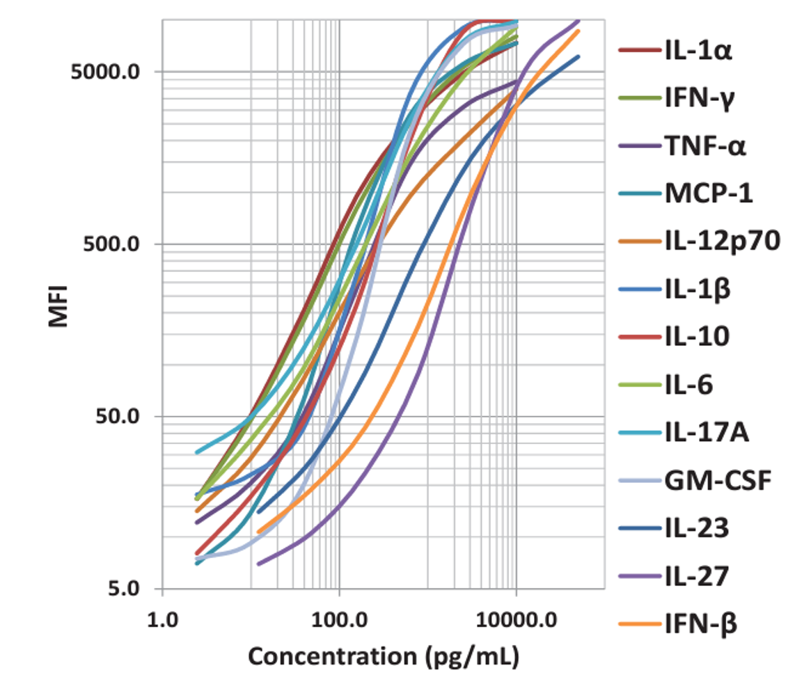 |
| This standard curve was generated using the LEGENDplex™ Immune Response Panel for demonstration purposes only. A standard curve must be run with each assay. |
|
Our immunoassays are validated for over 200 analytes, from individual and sandwich-based ELISAs to flow cytometry-based multiplex panels. Our pre-defined panels quantify up to 14 analytes and are designed for your research area. Alternatively, our custom solutions team can build custom panels with your analytes of interest.
Linear and logistic regressions are the two most commonly used curve-fitting models for sandwich immunoassays. Although linear regression may be useful when analyzing samples that fall within the linear portion of the response curve, logistic regression is the preferred regression type for multiplex immunoassays. |
| Traditional sandwich ELISAs and bead-based multiplex immunoassays, such as LEGENDplex™, are frequently used to detect and quantify specific analytes within a biological sample. These samples include serum, plasma, cell culture supernatants, and other biological matrices. In order to determine the concentration of an analyte within a sample, one must run a standard, or calibration, curve. The production of a standard curve requires the use of known concentrations of the analyte being assayed. Performing a quantitative immunoassay asks one to plot an x-y plot that shows the relationship between this standard (analyte of interest) with the readout of the assay, e.g. optical density (OD) for ELISA and mean fluorescence intensity (MFI) for LEGENDplex™. The concentration of the analyte in the sample can then be calculated using the OD or MFI. |
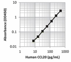 |
| This standard curve was generated using the LEGEND MAX™ Human CCL20 ELISA Kit for demonstration purposes only. A standard curve must be run with each assay. |
|
Before samples can be analyzed, it is important to choose the best curve fit model to achieve the most accurate and reliable results. Thankfully, you can use our free LEGENDplex™ Data Analysis Software Suite, and the analysis will be done for you and you do not need to use all of the formulas discussed later in the blog. However, they are important for understanding what curve to choose for your analysis. |
Linear Regression and Sum of Squared Residuals |
| The most straightforward way to analyze your immunoassay data is to use a linear regression curve fit. This generally means plotting the concentration vs. the assay readout (OD for ELISA or MFI for LEGENDplex™) and using the standard equation, y = mx + b The concentration is generally represented as x, the assay readout as y, with m referring to the slope and b referring to the y-intercept where x = 0. |
 |
| The aim is to find values for the slope (m) and y-intercept (b) that minimize the absolute distance from the data point to the curve, also known as the residual. |
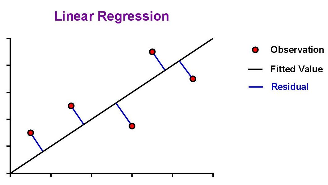 |
| The ideal assumption is that the best-fit linear curve will be a line that passes as close as possible to all data points from the standard curve. The question that arises from this is, "How is this assessed?" This is where the concept of a 'residual' is introduced. Since the best fit line will be the one that passes closest to all data points, it should seem natural that we could simply sum the residuals of all data points and the line with the lowest sum would be the best. |
|
However, there is an underlying problem here that needs to be addressed. Take an over-simplified example where we are looking at residuals from just 2 data points, A & B. Now, imagine we fit 2 linear curves to the data. The first gives residuals of A = 1 and B = 9, and the second gives A = 5 and B = 5. If we sum the residuals, both curves give the same answer of 10. This is problematic since mathematically they are "equivalent", but clearly the second curve fits the data better as it passes closer to both data points. More simply put, 5 for each is a better fit than 1 and 9. |
|
The solution to this issue is to square the residual values first, and then add them together. By transforming the data like this, curves with poorer fits and larger residuals will be scored higher and become less desirable. To revisit the example from above, 52 + 52 = 50, and 12 + 92 = 82. Rather than being mathematically equivalent, now the better fit curve has the lower sum of squared residuals. |
| This is referred to as sum of squared residuals, and the smaller this number is, the better the curve fit your data. |
| However, since immunoassays are used for biological measurements, they almost never follow a linear response. In fact, the instruments that we use to measure these responses (OD, MFI, etc.) also have upper limits. Therefore, due to the complex nature of the biological systems being assayed, a more complex form of modeling must be used. Due to the complex nature of the biological systems being assayed, a more complex form of modeling must be used. |
Non-linear Curve Models: 4-Parameter Logistic (4PL) |
| Immunoassay standard curves typically produce an S-shaped sigmoidal curve, which requires a different kind of mathematical modeling called logistic regression, that allows for curve fitting beyond the linear range of the curve. This new range is referred to as the logistic range, and is most simply described by a 4PL curve. This type of modeling still uses the underlying concept of summing the square of the residuals, but instead of minimizing residuals for a straight line, we're now doing so with an S-shaped curve that is defined by the following parameters. | 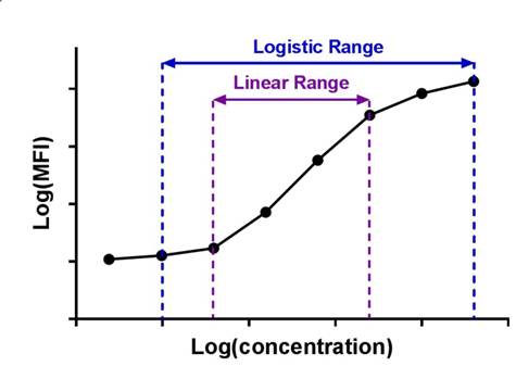 |
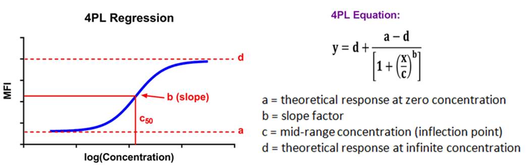 |
| This type of analysis uses an equation that has a maximum and minimum incorporated into it, and 4 parameters, hence the name. If your data produces a symmetrical, S-shaped curve, a 4PL fit should be sufficient to analyze your data. |
Non-linear Curve Models: 5-Parameter Logistic (5PL) |
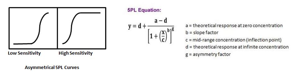
| At times when running an ELISA, or more complex multiplexing assays such as LEGENDplex™, you may not get a symmetrical curve. To remedy this, there is an additional parameter that can be added to the 4PL equation, thus allowing one to do a 5PL curve fit. This fifth parameter takes into account an asymmetry factor, g, and provides a better fit when the curve does not have symmetry. |
 |
How Well Does Your Model Fit Your Data? |
|
Using the appropriate curve fitting model is important for generating reliable, high quality data. The "goodness of the curve fit" refers to how well a curve fits the data that has been generated. Linear regression uses the R2 value as a good representation of the "goodness of fit". A curve is considered to have a very good fit when the R2 value is over 0.99. |
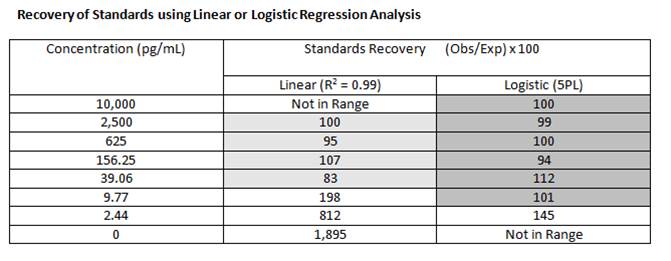
Recovery of Standards |
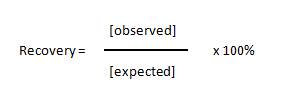
| The recovery of standards allows one to measure the accuracy of the observed concentration that was calculated for the expected concentrations of each standard. Basically, you calculate the concentration of each standard and compare it to the actual concentration using the following equation: |
 |
|
The closer the recovery is to 100%, the better the curve fit model being used. The general rule of thumb says for accurate quantification, the recovery should fall between 80-120%. Using logistic regression (4PL or 5PL), rather than linear regression, will allow for more accurate quantitation across a wider range. |
 |
Spike and Recovery |
|
Spike and recovery is used to test the accuracy of your assay. Spike and recovery experiments are generally used to assess if your sample matrix (plasma, serum, etc.) is causing interference with the ability of the capture and detection antibodies to bind to the target protein being assayed. By adding, or "spiking", a known concentration of the recombinant standard into your sample and comparing this to the same concentration of recombinant spiked into the standard diluent, or blank, you can assess whether anything in your sample matrix is causing interference. You should always include your sample with no spiked recombinant so you are able to measure any endogenous protein that may already be there. All three of these samples are measured and concentrations are determined relative to the standard curve. As with the standard recovery, your spike recovery should also fall between 80-120%. |
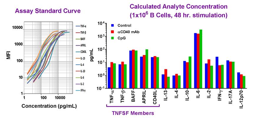 |
| Example dataset and standard curve generated using the LEGENDplex™ Human B Cell Panel for demonstration purposes only. Standard curve must be run with each assay. Data (right) shows simultaneous quantification of key cytokines in B cells after 48 hr stimulation with αCD40 mAb (red) and CpG (green). |
|
Our featured LEGENDplex™ Human B Cell Panel is a bead-based multiplex assay panel that quantifies 13 key targets involved in B cell function, activation, proliferation, and survival. It allows simultaneous quantification of 13 human cytokines, which include: TNF-α, IL-2, IL-4, IL-6, IL-10, IL-12p70, IL-13, IL-17A, APRIL, BAFF, CD40L, IFN-γ, and TNF-β, and are collectively secreted by Be1, Be2, Breg, CD4+ T lymphocytes, dendritic cells and monocytes. This panel has been validated for use on cell culture supernatant, serum, and plasma samples. |
Summary |
|
The most common curve fitting models used for ELISAs and multiplexing immunoassays are linear regression and logistic regression. As discussed, the results for biological assays may not fall within the linear portion of the curve, so the need for logistic regression analysis such as 4PL or 5PL is almost always recommended. In our free LEGENDplex™ Data Analysis Software Suite, the default is 5PL. However, the user can opt to use a 4PL fit. In general, the 5PL algorithm provides the best fit regression line to assay data. In addition, the software evaluates the standard curve data using both the 5PL and 4PL algorithms, and then performs a statistical test comparing the goodness of fit for each of the regression lines (F-test comparing the residuals at each standard curve point for each algorithm). If the p-value derived is < 0.05, the 5PL algorithm should be used. If the p-value is non-significant, then either algorithm can be used.
Analyze your immunoassay data with confidence with our resources for ELISA and multiplex immunoassays. Learn how our complimentary LEGENDplex™ Data Analysis Software Suite analyzes flow cytometry data. |


Follow Us